
Safety Stock Calculation: Formulas, Methods, and Examples
The two formulas you need are the Max–Min (basic) and the statistical Z-score formula. Use Max–Min when you have limited history or are protecting C-items; use the statistical formula for A-items with at least 90 days of reliable demand and lead-time data.
The two core formulas:
- Max–Min (basic): Safety Stock = (Max Daily Demand × Max Lead Time) − (Avg Daily Demand × Avg Lead Time)
- Statistical (full form): SS = Z × √(L × σD² + Davg² × σL²)
- Statistical (simplified, stable lead time): SS = Z × σD × √L
Minimum inputs for each:
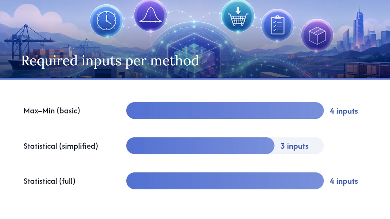
- Max–Min: max daily demand, max lead time, average daily demand, average lead time
- Statistical (simplified): Z-score for your service level, σD (demand standard deviation), average lead time L
- Statistical (full): all of the above plus σL (lead-time standard deviation)
The Max–Min formula is conservative by design. It assumes the worst case simultaneously hits demand and lead time, so it tends to overstock. The statistical formula is more precise but requires clean data. If your demand history is patchy or your supplier lead times are inconsistently recorded, start with Max–Min and migrate to the statistical method as your data matures.
Key Takeaways
The most effective safety stock calculation matches formula complexity to your data quality and SKU criticality: use the statistical full formula for A-items, Max–Min for C-items, and recalculate on a defined schedule.
| Point | Details |
|---|---|
| Match method to data quality | Use Max–Min for limited data or C-items; use the full statistical formula for A-items with reliable variance data. |
| Measure inputs correctly | Compute σD and σL from actual transaction data, not quoted lead times or aggregated demand. |
| Connect safety stock to ROP | ROP = (Avg daily demand × Avg lead time) + Safety stock; omitting either term causes systematic reorder errors. |
| Service level is a cost tradeoff | Moving from 95% to 99% service level often requires roughly 40% more safety stock; justify it against stockout cost. |
| Recalculate on a schedule | Recalculate monthly for volatile A-items, quarterly for stable B-items; trigger an immediate recalc on any lead-time shift above 20%. |
Table of Contents
- What safety stock actually does for your operations and cash
- How to measure and compute every input you need
- Which safety stock calculation method fits your situation
- Worked example: Max–Min vs. statistical, with Excel formulas
- How safety stock feeds your reorder point and inventory policy
- Choosing service level and method: what the evidence says
- Common mistakes that make safety stock behave unexpectedly
- A practical plan for putting this into action
- How Usiship helps you reduce lead-time variability and carrying costs
- Sources
What safety stock actually does for your operations and cash
Safety stock is the buffer inventory you hold above your expected cycle stock to absorb demand spikes and supply delays without stocking out. It sits at the intersection of two competing pressures: the cost of a stockout (lost sales, expediting fees, customer churn) and the cost of carrying excess inventory (capital tied up, storage fees, obsolescence risk).
Cycle stock is what you consume in normal operations between replenishment orders. Safety stock is what you draw on when reality deviates from the plan. The two together determine your reorder point.
A practical way to see the tradeoff: a distributor holding 5 days of safety stock on a $50 unit moving 200 units per day carries $50,000 in buffer inventory. Cut that to 2 days and you free $30,000 in working capital but accept a much higher stockout probability during any supplier delay. The right number depends on your service-level target, your supplier’s reliability, and how much demand variability you actually see, not on a gut-feel “weeks of supply” rule.
- Safety stock protects customer service levels during demand and supply uncertainty.
- It is distinct from cycle stock, which covers normal replenishment cycles.
- It feeds directly into the reorder-point formula, so an error in safety stock cascades into a wrong reorder trigger.
- Too little means stockouts; too much means cash locked in shelves.
How to measure and compute every input you need
Getting the inputs right matters more than picking the “best” formula. A precise formula fed bad data produces a confidently wrong answer.
Average daily demand (Davg)
Pull your sales or consumption data for the past 90–180 days for stable SKUs. For volatile or seasonal SKUs, use a shorter window (30–60 days) weighted toward recent periods.
=AVERAGE(B2:B181) where column B holds daily units sold.
Standard deviation of demand (σD)
=STDEV.S(B2:B181) on the same daily demand range. If your system exports weekly data, convert to daily standard deviation by dividing by √7: =STDEV.S(range)/SQRT(7).
Average lead time (L) and lead-time standard deviation (σL)
Track actual PO-to-receipt days for each purchase order over the past 6–12 months. Most ERP systems (SAP, Oracle, NetSuite) store receipt dates against PO dates; export that table and compute:
=AVERAGE(C2:C51)for average lead time across 50 POs=STDEV.S(C2:C51)for σL
Lead-time variability often dominates safety-stock requirements, so tracking actual PO-to-receipt times rather than using a supplier’s quoted lead time is worth the extra data work.
Service level and Z-score
Service level is the probability of not stocking out during a replenishment cycle. You choose it based on the cost of a stockout versus the cost of carrying more inventory. Common Z-scores:
Pro Tip: Pull demand data from your WMS or ERP at the SKU-location level, not the aggregate. Aggregated demand hides the variability that drives safety stock. For 90–180 days of stable SKUs, daily granularity is ideal; for volatile SKUs, 30–60 days of daily data often captures the relevant pattern better than a longer window that includes structural demand shifts.
Which safety stock calculation method fits your situation
There is no universal safety stock formula; the right choice depends on your data quality and SKU criticality. Applying a complex statistical model to a C-item with two years of patchy data produces a misleading result. Applying a simple fixed-days rule to your top revenue SKU leaves money and service on the table.
Here is how the main methods stack up:
| Data Required | Recommended Method | Typical SKU Type |
|---|---|---|
| Max demand, max lead time, averages only | Max–Min (basic) | C-items, new SKUs, limited history |
| σD, average L (stable supplier) | Statistical simplified: Z × σD × √L | B-items, moderate data quality |
| σD, average L, σL | Statistical full: Z × √(L × σD² + Davg² × σL²) | A-items, high-value, variable lead time |
| Fixed policy, no variance data | Fixed days of supply (e.g., 7-day rule) | Low-value, non-critical, stable demand |
Max–Min (basic) formula
Formula: SS = (Max Daily Demand × Max Lead Time) − (Avg Daily Demand × Avg Lead Time)
Covers worst-case demand and worst-case lead time simultaneously. No standard deviation required. It is conservative, so it tends to overstock, but that is acceptable for C-items or when you are starting from scratch. Use it when you have fewer than 30 data points or when preventing any stockout is the priority regardless of carrying cost.
Statistical simplified (demand variability only)
Formula: SS = Z × σD × √L
Assumes lead time is stable and only demand fluctuates. Faster to compute and works well when your supplier is reliable. A good fit for B-items where you have solid demand history but lead times rarely vary.
Statistical full form (demand + lead-time variability)
Formula: SS = Z × √(L × σD² + Davg² × σL²)
The most accurate method when both demand and lead time vary. Required for A-items with variable suppliers. More data-intensive but produces a tighter, more defensible buffer.
Fixed days of supply
A rule-of-thumb approach: hold X days of average demand as safety stock. Simple to communicate and implement. Appropriate for low-value, non-critical items where the cost of a sophisticated calculation exceeds the value of the precision.
Heizer and Render variant
Uses maximum expected demand and maximum lead time in a slightly different form, sometimes expressed as SS = (Max daily demand − Avg daily demand) × Lead time. Produces a result between the Max–Min and statistical methods. Useful when you want to avoid full statistical computation but need something more nuanced than the pure Max–Min.
Worked example: Max–Min vs. statistical, with Excel formulas
SKU data for this example:
- Average daily demand (Davg): 50 units
- Standard deviation of demand (σD): 10 units
- Average lead time (L): 14 days
- Standard deviation of lead time (σL): 3 days
- Maximum daily demand: 70 units
- Maximum lead time: 21 days
- Unit cost: $25
- Service level: 95% (Z = 1.645)
Step-by-step calculations
A. Max–Min formula
- Max Daily Demand × Max Lead Time = 70 × 21 = 1,470 units
- Avg Daily Demand × Avg Lead Time = 50 × 14 = 700 units
- Safety Stock = 1,470 − 700 = 770 units
Excel: =(D2*F2)-(B2*D4) where D2 = max demand, F2 = max lead time, B2 = avg demand, D4 = avg lead time.
B. Statistical full formula
- L × σD² = 14 × (10²) = 14 × 100 = 1,400
- Davg² × σL² = (50²) × (3²) = 2,500 × 9 = 22,500
- Sum = 1,400 + 22,500 = 23,900
- √23,900 ≈ 154.6
- SS = 1.645 × 154.6 ≈ 254 units
Excel: =NORM.S.INV(0.95)*SQRT((D4*(C2^2))+(B2^2*(E2^2))) where C2 = σD, E2 = σL.
Comparison of results
The Max–Min method holds $12,900 more in buffer inventory for this single SKU. Across a catalog of 500 A-items, that gap compounds fast. The statistical formula earns its complexity for high-value, high-volume SKUs precisely because the carrying-cost savings are material.
Pro Tip: Build a single Excel tab with named ranges for each input (Davg, σD, L, σL, Z) and reference them in both formula cells. When you update one input, both methods recalculate instantly. Add a third column for ROP using =B2*D4+SS_cell so your reorder trigger updates automatically.
How safety stock feeds your reorder point and inventory policy
The reorder point formula is: ROP = (Average Daily Demand × Average Lead Time) + Safety Stock

The first term covers expected consumption during the replenishment period. Safety stock covers the deviation from that expectation. If you calculate safety stock correctly but set ROP using only the demand-times-lead-time term, you will routinely dip into your buffer for normal replenishment, which defeats its purpose.
Continuous vs. periodic review
- Continuous review (fixed reorder point): You monitor inventory in real time and place an order whenever stock hits the ROP. Safety stock covers variability only during the lead time. This is the standard model for the formulas above.
- Periodic review (order-up-to): You check inventory at fixed intervals (weekly, monthly) and order up to a target level. Safety stock must cover variability during both the review period AND the lead time, so it is always larger than in a continuous-review system for the same service level.
For periodic review, adjust the lead time in your formula to L + T, where T is the review interval in days. A weekly review with a 14-day lead time means you calculate safety stock as if lead time were 21 days.
- Shorter review periods reduce safety stock requirements.
- Larger lot sizes can mask stockout risk between reviews.
- Supplier reliability directly affects how much buffer you need; improving lead-time consistency through better carrier relationships reduces σL and therefore required safety stock.
Choosing service level and method: what the evidence says
The choice of service level is an economic decision, not a default. Moving from a 95% to a 99% service level often requires roughly 40% more safety stock, which means 40% more capital tied up in buffer inventory for that SKU. That cost must be weighed against the actual cost of a stockout: lost margin, expediting fees, customer penalties, or brand damage.
Service-level Z-score reference
SKU segmentation guidance
Practitioners should apply statistical formulas to A-items and simpler, conservative methods to C-items to avoid wasting analytical effort and cash on low-value SKUs. A practical segmentation:
- A-items (top 20% of revenue or criticality): Use the full statistical formula. Set service level at 97–99%. Recalculate monthly.
- B-items (next 30%): Use the simplified statistical formula (stable lead time assumed). Set service level at 95%. Recalculate quarterly.
- C-items (remaining 50%): Use Max–Min or a fixed days-of-supply rule. Set service level at 90%. Recalculate semi-annually or when a stockout occurs.
Recalculation cadence and monitoring signals
Safety stock levels should be recalculated regularly because demand patterns and lead times shift. Static safety stock set once and forgotten will either overstock or understock within a few months.
Watch for these signals:
- Safety stock untouched for 3 or more consecutive replenishment cycles: your buffer is too high; reduce it.
- Repeated stockouts despite holding safety stock: your inputs are stale or your formula underestimates variability; recalculate.
- A supplier lead-time change of more than 20%: recalculate immediately regardless of schedule.
Pro Tip: Integrating supplier lead-time data and production scheduling visibility into your safety-stock model can reduce required buffer by 20–40% because much of what looks like demand randomness is actually operational uncertainty you can address at the source. Share rolling forecasts with key suppliers and track actual vs. quoted lead times monthly.
Common mistakes that make safety stock behave unexpectedly
Most safety-stock problems trace back to a handful of recurring errors. Here is where things go wrong and how to fix them.
-
Applying one formula to every SKU. A single method applied catalog-wide either overstocks C-items or understocks A-items. Segment by ABC class and match method to criticality.
-
Using weeks-of-supply as a proxy. “Hold two weeks of safety stock” sounds simple but ignores actual demand variability. A SKU with low average demand but high variance needs more buffer than a high-average, low-variance SKU at the same weeks-of-supply level.
-
Ignoring lead-time variability. Using only the simplified formula (Z × σD × √L) when your supplier’s lead time swings by 5–7 days understates safety stock significantly. Check σL before choosing the simplified vs. full formula.
-
Stale inputs. Demand patterns shift. A safety stock calculated on last year’s data may be wrong today. Build a calendar reminder to recalculate on schedule.
-
Aggregating demand data. Running the formula on total warehouse demand rather than SKU-location demand hides the variability that drives stockouts at specific locations.
-
Confusing safety stock with reorder point. Setting ROP equal to safety stock means you are ordering only when you have already consumed your buffer. ROP must include the demand-during-lead-time term.
-
Not tracking actual lead times. Using a supplier’s quoted lead time instead of measured PO-to-receipt times understates σL and produces a false sense of precision.
Quick fixes you can implement this week: re-pull demand data at the SKU-location level, verify that your ROP formula includes both terms, and check whether your lead-time inputs are measured or quoted.
Changes that require system or supplier work: setting up automated PO-to-receipt tracking in your ERP, establishing a shared forecast with key suppliers, and building a scheduled recalculation workflow in your planning system.
A practical plan for putting this into action
Most teams stall on safety stock because they try to perfect the model before acting. The better move is to get a defensible number for your top SKUs this week and refine from there.
This week:
- Pull 90–180 days of daily demand data for 5 A-items and 5 C-items from your ERP or WMS.
- Compute Davg and σD in Excel using
=AVERAGE()and=STDEV.S(). - Pull the last 20–50 POs for those SKUs and compute average lead time and σL.
- Run both the Max–Min and statistical formulas side by side. Note the gap.
- Flag any SKU where safety stock in your system differs from your calculated result by more than 20%.
This month:
- Run the full statistical formula for all A-items. Update ROPs in your system.
- Set a review calendar: monthly recalculation for volatile A-items, quarterly for B-items.
- Meet with your top 3 suppliers to validate quoted vs. actual lead times and share a 90-day rolling forecast.
- For C-items, apply the Max–Min formula or a fixed 7-day rule and move on. Don’t spend A-item analytical effort on C-items.
The goal is a working model that gets recalculated on schedule, not a perfect model that never gets built.
How Usiship helps you reduce lead-time variability and carrying costs
Accurate safety stock calculations depend on reliable lead times. When suppliers are inconsistent and transit times vary, σL climbs and your required buffer grows with it. One of the most direct ways to reduce safety stock is to reduce the variability in your supply chain, not just measure it better.
Usiship’s customs clearance services reduce the unpredictability that imported SKUs introduce into lead-time calculations, a common driver of inflated safety stock for businesses sourcing internationally. For businesses managing high-value or specialty inventory, Usiship’s warehouse solutions provide the inventory accuracy and storage practices that make safety-stock calculations actually reflect what is on the shelf. And for e-commerce operators managing safety stock across multiple channels, omnichannel fulfillment services from Usiship give you the visibility to set and monitor reorder points without manual reconciliation.